Animation
inbetweening

return to main index

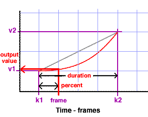
Introduction

Inbetweening is a technique for calculating values that change systematically during an animation. Generally, it will be known over which (key) frames in an animation an output value will change. The diagram shown below is a simplified version of the type of information displayed by an animation editor available in all 2D/3D applications.

Figure 1

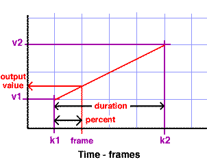
The known values are shown in purple and those that will be calculated are shown in red. k1 and k2 are the keyframes at which the output value begins and ends its change. frame is the current frame at which the output value will be calculated. v1 and v2 are the min and max values for the output. Since the output value will change smoothly, shown by the straight diagonal red line, this type of inbetweening is called linear inbetweening.

General Method

The easiest way of understanding the calculation of an output value is to look at an example. Suppose we have an output value that will be used to set the radius of a circle or sphere. Lets say at the beginning and end of the animation the radius should be 1.5 and 4.5. Therefore,

Also lets say the frames at which the radius begins and ends its change are 10 and 40, therefore,

Finally, lets calculate what the output value ie. radius, will be at, say, frame = 20. At this frame we are a certain percentage of the way from keyframe 1 to keyframe 2 ie.

We can use the percent value to find by how much the output value ie. the radius, has changed from its min to its max value.

The 'C' code for performing linear inbetweening is shown in listing 1.

Listing 1 (inbetween.c)

#include <stdio.h>
#include <math.h>
  
void main()
{
int    frame = 20, k1 = 10, k2 = 40;
float  v1 = 1.5, v2 = 4.5;
float  percent, radius;
  
if(frame < k1)
    radius = v1;
else if(frame > k2)
    radius = v2;
else       
    {
    percent = (float)(frame - k1)/(k2 - k1);
     radius = (v2 - v1) * percent + v1;
    }
printf("radius at frame 20 is %1.3f \n", radius);
}

Because frame numbers are integers it is necessary to do the cast or promotion at line 16. Without the "if" and "else if" on lines 10 to 13 the incorrect values of radius would be calculated.

A Tcl version of this calculation is shown in listing 2.

Tcl Implementation

A Tcl implementation for linear inbetweening is shown below.

Listing 2 (inbetween.py)

set v1 1.5
set v2 4.5
 
set frame 20.0
set k1 10
set k2 40
  
set {$frame < $k1} {
    set radius $v1
} set {$frame > $k2} {
    set rad $v2
} set {
    set percent [set $frame - $k1]
    set percent [set $percent / [set $k2 - $k1]]
     set radius [set [set [set $v2 - $v1] * $percent] + $v1]
    }
set "radius at $frame is $radius"

Acceleration

The animation of many phenomena require that changes occur in an accelerating or deaccelerating fashion. For example, take an exploding fireworks "sky rocket" that forms a spherical shell of colored sparks.

Figure 2

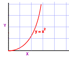
The rate at which its radius increases will deaccelerate as the material forming the sparks loses momenentum. Using linear inbetweening to determine the radius of the explosion would be wrong. A typical acceleration curve is shown in figure 2 where an output value, Y, is determined by an input value, X, multiplied by itself.

Figure 3

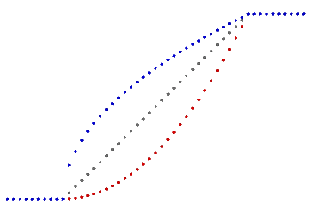
As shown above, using such a curve gives a different output value than the linear interpolation, shown by the gray line. Therefore, line 16 of the 'C' implementation, where the percent value is calculated ie.

should be changed to,

But what about de-acceleration?

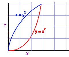
De-acceleration

A typical acceleration curve is shown on the right in blue. The equation for the deacceleration can be re-written as,

Likewise, the 'C' maths function pow() could also be used for the acceleration,

If the second value of pow() is made equal to 1.0 we have a linear relationship between the x and y values. When the second value become the reciprocal of 2 ie. 0.5 we have the de-acceleration curve shown in blue. If however, the second value becomes zero ie.

the 'y' value stays at 1.0. Listing , a 'C' implementation of an inbetweening is given in listing 3.

Figure 4

Listing 3

float tween(int k1, int k2, int frame, 
           float v1, float v2, float rateOfChange)
{
float  percent, output;
  
if(frame < k1)
    output = v1;
else if(frame > k2)
    output = v2;
else       
    {
    percent = (float)(frame - k1)/(k2 - k1);
    percent = (float)pow(percent, fabs(rateOfChange));
     output = (v2 - v1) * percent + v1;
    }
return output;
}

A Tcl implementation of this function is given in listing 4.

Listing 4

proc tween {k1 k2 frame v1 v2 rateOfChange} {
if {$frame < $k1} {
    set output $v1
} elseif {$frame > $k2} {
    set output $v2
} else {
    set percent double([expr $frame - $k1])
    set percent [expr $percent / [expr $k2 - $k1]]
    set percent [expr pow($percent, $rateOfChange)]
    set output [expr [expr [expr $v2 - $v1] * $percent] + $v1]
    }
return $output
} 

The main problem with this function is that both for acceleration and de-acceleration the final output value ie. v2 is reached abruptly.

Figure 5