Rsl - Blobby Effects

RSL
Blobby Effects

Introduction

Blobby objects, otherwise known as soft objects or implicit surfaces, enable fluid effects, such as water separating into droplets, to be modeled and animated. This tutorial does not deal with RenderMan's Blobby RIB statement but instead shows how the general principles of implicit surfaces can be applied to surface shading.

Some modeling applications, such as Maya, support a type of object called a blobby. RenderMan supports such objects via a Bobby RIB statement. For details refer to PhotoRealistic RenderMan Application Note #31. It can be found within the Pixar installation at,

Blobby Implicit Surfaces

In general, blobby (3D) objects are defined by at least three attributes,

a center point - a single xyz location
a radius, and
a value of some kind that is constant over their surface.

The center point defines the location from which a blobby radiates a field (of values). Much in the same way as a point source of illumination radiates light, the strength of the field surrounding a blobby diminishes away from its center. Eventually, the strength of the field drops to zero at some predefined radius.

In the case of a 3D blobby object its spherical surface is drawn where the field values around its center share the same value. For this reason blobby objects are also known as iso-surfaces; "iso" means equal.

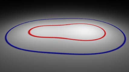
Figure 1

For example, the polygon shown in figure 1 is illuminatd by two point lights. Naturally, we see the gradation of brightness across its surface. However, if those parts of the polygon that share the same level of illumination are connected with a colored line the polygon is, in effect, displaying a slice through an otherwise invisible halo ie. field, of equal brightness values. In figure 1 the red line connects all the points on the surface of the polygon that share an intensity of 1.2 while the blue line passes through intensity values of 0.3.

Unlike point light sources whose field of illumination diminishes somewhat abruptly, most modelling/rendering systems that support blobby objects use fields that diminish less abruptly - figure 2. This tutorial shows how blobby-like effects can be utilized by surface and displacement shades.

Figure 2

Basic Code

The code in listing 1 applies the principle of a blobby object to a surface shader. Simple_blobby has three parameters that control its blobby effect. The iso parameter controls the size of the blobby patch that it applies to a surface. The arrays contain the xyz location of three blobbies and their radii.

Listing 1

surface
simple_blobby(float    Kd = 1,
                       iso = 0.5;
              float    rad[3] = { 1.0,0.6,1.5};
              point    pnt[3] = { (-0.95,0,0),(0.1,0,1.2),(0.85,0,0) };
             )
{
normal   nf, n;
color    diffusecolor, surfcolor = Cs;
point    p;
  
/* STEP 1 - make a copy of the surface normal one unit in length */
n = normalize(N);
nf = faceforward(n, I);
  
/* STEP 2 - set the apparent surface opacity */
Oi = Os;
  
float totalfield = 0, dist;
uniform float j;
/* STEP 3 - use the smoothstep function to generate a combined
            field value based on the distance to each blobby */
for(j = 0; j < 3; j = j + 1)
    {
    p = transform("current", pnt[j]);
    dist = distance(P, p);
    totalfield += 1 - smoothstep(0, rad[j], dist);
    }
/* STEP 4 - assign a color to the surface if the current location
            being shaded is within the target iso value */ 
if(totalfield > iso)
    surfcolor = color(1, 0, 0);
        
/* STEP 5 - calculate the diffuse lighting */
diffusecolor = Kd * diffuse(nf);
  
/* STEP 6 - calculate the apparent surface color */
Ci = Oi * Cs * surfcolor * diffusecolor;
}

The shader uses the smoothstep() function to generate a smoothly changing field value for each blobby based on its distance from the current shading point P. Because xyz's of each blobby are measured in the world coordinate sytem while the xyz of the point (P) being shaded are measured in another coordinate system the shader converts each blobby xyz to the "current" coordinate - which is almost certainly the camera coordinate system. Listing 2 shows how the "simple_blobby" shader is used on a polyplane.

Listing 2

Display "blobby_tester" "framebuffer" "rgb"
Format 427 240 1
Projection "perspective" "fov" 40
ShadingRate 1
  
Translate  0 0.35 3
Rotate -30 1 0 0
Rotate 0   0 1 0
Scale 1 1 -1
  
WorldBegin
    LightSource "pointlight" 1 "float intensity" 50 
                "point from" [1 4 1]
  
    TransformBegin
        Declare "pnt" "point[3]"
        Declare "rad" "float[3]"
        Surface "simple_blobby"
                "pnt" [-0.95 0 0   0.1 0 1.2   .85 0 0]
                "rad" [1   0.6   1.5]
                "float iso" 0.3
        Polygon "P" [-0.5 0 -0.5   0.5 0 -0.5  
                      0.5 0 0.5  -0.5 0 0.5]
                "st" [0 0  1 0  1 1  0 1]
    TransformEnd
WorldEnd

Figure 3

The basic shader can be improved and made to generate more interesting effects in several ways. Its principle weakness is that it uses a simple "if" test to decide whether or not to apply red to the surface. This binary decision inevitably produces serious aliasing artifacts - note the jagged perimeter of the blobby coloration in figure 3.

Smoothing

Rather than using an "if" test the code in listing 3 uses a combination of smoothstep() and mix(). In the "zone" 0.05 either side of the target iso value the function returns a "blend" value that change smoothly betwee 0 and 1. Subsequently, blend is used to control the color mixing. The enlarged view in figure 4 shows the edge of the blobby smoothed or antialiased.

Listing 3

/*
if(totalfield > threshold)
    surfcolor = color(1, 0, 0);
*/
float blend = smoothstep(iso-0.05,iso+0.05,totalfield);
surfcolor = mix(Cs, color(1,0,0), blend);

Figure 4

Ideally, the explicit value of 0.05 should be substituted for a shader parameter so that the degree of smoothing can be set by the rib file.

Blobby Contours

A "contour" line can be rendered by multiplying two smoothsteps - figure 5.

Listing 4

float blend = smoothstep(iso-0.05,iso,totalfield) *
         (1 - smoothstep(iso,iso+0.05,totalfield));
surfcolor = mix(Cs, color(1,0,0), blend);

Figure 5

Blobby Polarity

In addition to their standard characteristics, blobbies can also be assigned polarity. In listing 5 we see that this version of the blobbies surface shader is passed an array of values indicating whether a particular blobby has a positive or a negative field.

Listing 5

for(j = 0; j < 3; j = j + 1)
    {
    p = transform("current", pnt[j]);
    dist = distance(P, p);
    if(polarity[j] == 1)
        totalfield += 1 - smoothstep(0, rad[j], dist);
    else
        totalfield -= 1 - smoothstep(0, rad[j], dist);
    }

Figure 6

Blobby Color

Bobbies can also be given an individual color. This version uses mixtures of colors to indicate where parts of a surface have been influenced by more than one blobby.

Listing 6

float    totalfield = 0, field, dist;
color    totalcolor = 0;
uniform float j;
for(j = 0; j < 3; j = j + 1)
    {
    p = transform("current", pnt[j]);
    dist = distance(P, p);
    field = 1 - smoothstep(0, rad[j], dist);
    totalcolor += col[j] * field;
    totalfield += field;
    }
float r = comp(totalcolor, 0);
float g = comp(totalcolor, 1);
float b = comp(totalcolor, 2);
r /= 3;
g /= 3;
b /= 3;
setcomp(totalcolor, 0, (r > 1) ? 1 : r);
setcomp(totalcolor, 1, (g > 1) ? 1 : g);
setcomp(totalcolor, 2, (b > 1) ? 1 : b);
  
float blend = smoothstep(iso-0.05,iso+0.05,totalfield);
surfcolor = mix(Cs, totalcolor, blend);

Figure 7

Noisy Blobbies

Modifying dist with noise before it is used by smoothstep to calculate the field value has a dramatic effect - figure 8. Of course, rather than increasing the frequency of the noise by a fixed value (7) the shader should have an additional parameter to control the noise.

Listing 7

for(j = 0; j < 3; j = j + 1)
    {
    p = transform("current", pnt[j]);
    dist = distance(P, p);
    
    dist *= noise(transform("object", P) * 7);
    totalfield += 1 - smoothstep(0, rad[j], dist);
    }

Figure 8