RSL
Interior Shading & vpvolumes

return to main index

Introduction

The relatively new shading strategy called vpvolumes was introduced in prman 12. It offers a solution to the previously thorny problem of applying volumetric shading effects to the interior of irregular objects without the use of ray tracing. The following Pixar notes provide detailed information about this topic.

"A Tour of Ray-Traced Shading in PRMan"
    prman_technical_rendering/AppNotes/rayintro.html#interiorvp
  
"Shading Strategy"
    prman_technical_rendering/users_guide/attributes.html#shade_strategy
    
"Writing Fancy Atmosphere Shaders"
    prman_technical_rendering/AppNotes/appnote.20.html

"A Tour of Ray-Traced Shading in PRMan" provides examples of the use of a fog shader. The code for the fog shader is given in "Writing Fancy Atmosphere Shaders". For most people, trying to tease apart the inner workings of the fog shader usually engenders a state of, well, fog. Shortly after encountering "Trapezoidal integration" most readers quickly realize that making sense of Pixar's fog shader is unlikely to be easy - few are disappointed!

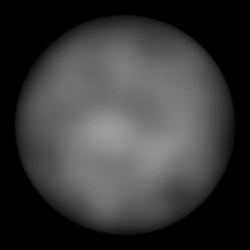
The purpose of this tutorial is to assist the reader in understanding how vpvolumes offer a convenient way of stepping along lines (vectors) that "connect" the front to the rear of an object. At each step, the shader calculates an arbitary, but consistent, value that it accumulates in order to modify the apparent surface color (Ci) and apparent surface opacity (Oi) of the micropolygon being shaded. In general, the values calculated at each step are derived from 3D noise and illumination.

Front and Rear

Figure 1 is based on an illustration accompanying, "Interior volume shaders without ray tracing"; a section of the first reference cited above. The sphere shown in the illustration has been assigned the following attribute.

    Attribute "shade" "strategy" ["vpvolumes"]

Figure 1

When a volume shader uses the global variable P it is accessing the micropolygon on the rear surface. Unlike a surface shader, an interior shader, does not shade the front surface. Another difference the vpvolumes shading strategy makes is that I "originates" at the front micropolygon, not at the origin of the camera coordinate system. Within a shader, points, vectors and normals are in camera space ie. they are "meaaured" from the origin of the camera. Consequently, the position of the front micropolygon is equal to P less the vector I ie.

    point     frontP = P - I;    // the "front" micropolygon

The distance from the front to back for a camera "ray" passing through a volume is,

    float     totalDist = length(I);

Stepping

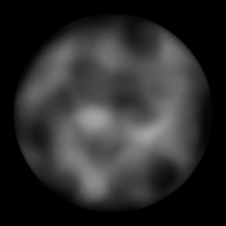
Figure 2 shows a few camera "rays" passing through a volume bounded by a sphere. At uniform intervals long each I vector an interior shader would, from front to rear,
    calculate the xyz position of each "step",
    use the xyz position to calculate (aka sample) one or more values,
    add the value/values to those previously calculated,
    assign the summed value/values to Oi and Ci.

Figure 2

The sphere shown above is 1.0 unit in diameter. Because the distance between the intervals (step size) was 0.2 the "ray" passing through the center of the sphere has 5 intervals along its length. The curved black lines represent the sample points for approximately 82,000 I vectors.

Basic Code

The basic code for an interior shader is shown below. Note the shader makes an initial randomized step before it begins sampling from front to rear. This ensures the volume is sampled in a way that avoids aliasing - figures 3, 4 and 5.

Figure 3
Randomized distribution of sample points

Figure 4
3D noise sampled uniformly

Figure 5
3D sampled using randomized points

Listing 1 - basic_interior.sl

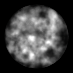
volume
basic_interior(float stepSize = 0.1)
{
float  totalDist = length(I);
float  numSteps = totalDist/stepSize;
point  frontP = P - I;    
point  currP = frontP;
float  accumulatedValue = 0;
  
// Jitter the starting distance
float  currDist = random() * stepSize;
  
while(currDist <= totalDist) {
    currP = frontP + currDist/totalDist * I;
    
    // Samples of one or more values are accumulated here...
    // accumulatedValue += ?
    
    // Prepare for the next iteration of the loop
    currDist += stepSize;
    }
// Modify the output colors.
Ci = Ci * accumulatedValue;
Oi = Oi * accumulatedValue;
}

Sampling 3D Noise

For simplicity the shader developed in this section samples 3D noise but does not make any lighting calculations.

Listing 2 - basic_noise.sl

volume
basic_noise(float stepSize = 0.05,
                  nFreq = 5,
                  nAmp = 0.05,
                  nMin = 0.45)
{
float   totalDist = length(I);
point   frontP = P - I;
point   currP = frontP, p;
float   accum = 0, ns;
float   currDist = random() * stepSize;
  
while(currDist <= totalDist) {
    currP = frontP + currDist/totalDist * I;
        
    // Simple sampling of 3D noise
    p = transform("current", "shader", currP);
    ns = noise(p * nFreq);
    accum += ns * nAmp;
    
    currDist += stepSize;
    }
Oi = accum;
Ci = accum;
}

Figure 6

The result of assigning the shader to a sphere is shown above. The lack of interior complexity combined with low contrast generates an uninteresting result.

Listing 3 - contrast_noise.sl

volume
contrast_noise(float stepSize = 0.05,
                     nFreq = 5,
                     nAmp = 0.065,
                     nMin = 0.48,
                     nMax = 0.65)
{
float   totalDist = length(I);
point   frontP = P - I;
point   currP = frontP, p;
float   accum = 0, ns;
float   currDist = random() * stepSize;
  
while(currDist <= totalDist) {
    currP = frontP + currDist/totalDist * I;
        
    // Simple sampling of 3D noise
    p = transform("current", "shader", currP);
    ns = noise(p * nFreq);
    accum += smoothstep(nMin, nMax, ns) * nAmp;
    
    currDist += stepSize;
    }
Oi = accum;
Ci = accum;
}

Figure 7

The use of smoothstep() provides a moderate degree of control over the contrast of neighboring regions of the interior. However, there is still a lack of interesting complexity within the volume.

Listing 4 - contrast_noise.sl

volume
noisey_fog(float stepSize = 0.05,
                 nFreq = 6,
                 nAmp = 0.16,
                 nMin = 0.4,
                 nMax = 0.85)
{
float   totalDist = length(I);
point   frontP = P - I;
point   currP = frontP, p;
float   accum = 0, ns;
float   currDist = random() * stepSize;
  
while(currDist <= totalDist) {
    currP = frontP + currDist/totalDist * I;
        
    // Three octaves of 3D noise
    p = transform("current", "shader", currP);
    ns = noise(p * nFreq);
    ns += (noise(p * nFreq * 2) - 0.5)/2;
    ns += (noise(p * nFreq * 4) - 0.5)/4;
    accum += smoothstep(nMin, nMax, ns) * nAmp;
    
    currDist += stepSize;
    }
Oi = accum;
Ci = accum;
}

Figure 8

The use of multiple overlays (octaves) of noise adds complexity to the interior.