RSL
Polar Coordinates & Famous Curves

return to main index

Related

    RSL: Archemedes Spiral

Introduction

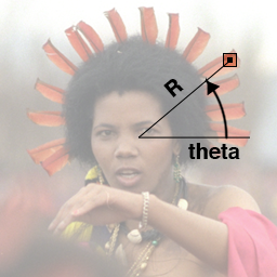
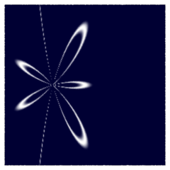
This tutorial looks at the basics of creating patterns defined within a 2D polar coordinate system. Using polar coordinates is somewhat unusual because the majority of effects applied by shaders generally depend on the direct use of 2D 'st' texture coordinates and/or the 3D coordinates of points, vectors and normals such as the global variables P, I and N. Before looking at the use of a 2D polar coordinate system this tutorial clarifies what are generically referred to as Cartesian coodinates.

Cartesian Coordinates

Locations within Cartesian coordinate systems are measured relative to the intersection of fixed coordinate axes that are perpendicular to each other. For example, figure 1 shows the coordinates (0.1, 0.45) of a point within a 2D Cartesian coordinate ('st' texture) system. Although 'st' texture space uses two perpendicular axes it does not mean they must be planar. 2D coordinate systems can be "drapped" around or over a curved surface.

Figure 1

Figure 2 shows the coordinates (1.0, 2.0, 0.7) of a point within a 3D Cartesian coordinate system.

Figure 2

2D Polar Coordinates

Figure 3 illustrates how the location of a point, within a polar coordinate system, is specified by distance (R) and angle (theta). In the shading language angles are measured in radians not degrees.

Figure 3

Relative to the center of the 1 x 1 polygon, shown in figure 3, the coordinates of the hilited box are,
    R = 0.4
    theta = 0.698 (ie. 40 degrees)
Since neither R or theta are global variables their values must be calculated by converting the 'st' (Cartesian) texture coordinates to their polar equivalents - listing 1.

Listing 1 - polar.h

void cartToPolar2D(float x, y, center, ycenter    
    output varying float R, theta)
{
float   xdiff = x - xcenter,
        ydiff = y - ycenter;
R = sqrt(xdiff * xdiff + ydiff * ydiff);
theta = atan(ydiff, xdiff);  // -PI to PI radians
theta = theta + 2 * PI;      //  0 to 2PI radians
}

Drawing Curves

The School of Mathematics and Statistics at the University of St.Andrews, Scotland maintains a web site of "Famous Curves". Many of the curves are defined by formula that require the use of polar coordinates. For example, figure 4 uses the polar description of a curve called the "Trisectrix of Maclaurin"

Figure 4 - output of the Maclaurin shader

Listing 2 provides the code for the shader that produced the pattern shown above. A sample rib file, listing 3, demonstrates the use of the shader.

Listing 2 - maclaurin.sl

surface
maclaurin(float Kfb = 1,        /* Fake brightness            */
                sc = 10,        /* [0.01 20] Scaling factor   */
                a = 2,          /* [0 10] Scaling factor      */
                b = 6,          /* [0 10] Lobes coefficient   */
                stroke = 0.03,  /* [0 1]  Lobes coefficient   */
                blur = 0.5,     /* [0 1] Softens the stroke   */
                scenter = 0.5,  /* [-2 2] Center in 's'       */
                tcenter = 0.5;  /* [-2 2] Center in 't'       */
        color   bakcolor = color(0,0,0.2),
                patcolor = 1    /* Color of the stroke        */
                )
{
float    R, theta;
float    ss = s * sc;
float    tt = t * sc;
  
// Convert the s,t location of the shading point 
// to polar coordinates.
float   xdiff = ss - scenter * sc, ydiff = tt - tcenter * sc;
R = sqrt(xdiff * xdiff + ydiff * ydiff);
theta = atan(ydiff, xdiff); // -PI to PI radians
if(theta < 0.0)
    theta += 2 * PI;        // 0 to 2PI radians
  
// Use the Maclaurin formula
float r = a * cos(b * theta)/cos(theta);
float blend = smoothstep(abs(R - r) - blur, 
                         abs(R - r), stroke);
Oi = Os;
Ci = Oi * mix(bakcolor, patcolor, blend) * Kfb;
}

Listing 3 - maclaurin.rib

Option "searchpath" "shader" "@:PATH_TO_USERS_SHADERS_DIR"
  
Display "maclaurin" "it" "rgb"
Format 240 240 1
Projection "perspective" "fov" 20
ShadingRate 1
  
Translate  0 0 3
Rotate -90 1 0 0
Rotate 0   0 1 0
Scale 1 1 -1
WorldBegin
    Surface "maclaurin"
            "float sc" 10
            "float a" 2
            "float b" 6
    Polygon "P" [-0.5 0 -0.5  -0.5 0 0.5  0.5 0 0.5  0.5 0 -0.5]
                "st" [0 0  0 1  1 1  1 0]
WorldEnd