RSL
Writing Surface Shaders


return to main index


Overview

This tutorial covers the basics of using the RenderMan Shading Language for the purpose of writing surface shaders. Several shaders are presented that can serve as starting points for the readers own explorations. The reader is encouraged to use the Cutter text editor for shader writing. Details of how it should be set up are given in the tutorial "Cutter Setup: RenderMan Shader Writing". This tutorial develops a series of variations of a basic constant shader. Finally, issues of diffuse lighting are addressed. The shading techniques used in this tutorial do not require ray tracing.


A Basic Surface Shader

Prior to shading an object a RenderMan complient renderer subdivides the surface of an object into mirco-polygons. The role of a surface shader is to determine the apparent surface opacity and color of each micro-polygon. The first set of shaders in this section are based on Cutter's "Constant" template surface shader.


To create a new shader document
select either "Diffuse" or "Constant"


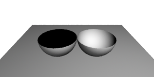
Although a constant shader does not consider the effect of lighting it is, nonetheless, a very good starting point for learning about shader writing.


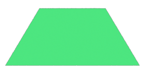
The Constant Color Shader


/* Shader description goes here */
surface
constant_test(float  Kfb = 1  /* fake brightness */)
{
color    surfcolor = 1;
  
/* STEP 1 - set the apparent surface opacity */
Oi = Os;
  
/* STEP 2 - calculate the apparent surface color */
Ci = Oi * Cs * surfcolor * Kfb;
}


In STEP 1 the apparent surface opacity is assigned the same value of the true surface opacity. In other words, this shader ensures a surface will conform exactly to the value of the Opacity statement in the rib file.

    Opacity 1 1 1    # this will define the value of "Os"
    Color   1 1 1    # this will define the value of "Cs"
    Surface "constant_test" "Kfd" 1
    Polygon "P" [data....]

The global variables that defines the apparent surface opacity and the true surface opacity are Oi and Os. Hence, the assignment,

    Oi = Os;

ensures that nothing fancy is being done to the opacity of an object.

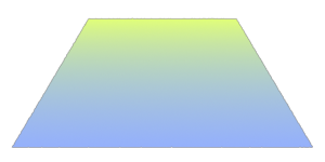
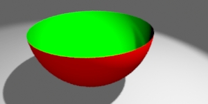
In STEP 2 the apparent surface color (Ci) is assigned the value of the true surface color (Cs) tinted by an internally defined variable called surfcolor. Colors are "combined" by their red, green and blue components being multiplied together. Color multiplication, filters (or tints) one color by another color. Because surfcolor is white ie. its rgb components are all equal to 1.0, it has no effect on the resulting color. In later examples, surfcolor will have a noticable effect on the final apparent color of a surface.

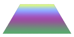
The multiplication by the apparent surface opacity (Oi) ensures the resulting color of each micro-polygon is pre-multiplied by its opacity. This enables the renderer to correctly composite the micro-polygons of foreground surfaces over micro-polygons of surfaces in the background.


Assigning a Color

Colors may be assigned as a single value (grayscale) or three individual (component) values, for example,

    color c;   /* declare a variable of data type color    */
    c = 0.8;                    /* grayscale color         */
    c = color(0.3, 0.9, 0.5);   /* assign a specific color */

"RGB" is the default color space. Listing 1 applies a pale green color to a surface.


Listing 1


surface
constant_test1(float  Kfb = 1)
{
color  surfcolor = color(0.3, 0.9, 0.5);
  
Oi = Os;
Ci = Oi * Cs * surfcolor * Kfb;
}


Figure 1 - a polygon of constant color


Adding Color Parameters

Two color parameters have been added to listing 2. The mix() function uses these colors to create a ramp based on the 't' texture coordinate.


Listing 2


surface
constant_test2(float    Kfb = 1;
                color   top = 1,
                        lower = 0)
{
color    surfcolor = mix(top, lower, t);
  
Oi = Os;
Ci = Oi * Cs * surfcolor * Kfb;
}

The Surface statement in the rib file that referenced the shader is shown below.

    Surface "constant_test2"
            "Kfb" 1.0
            "top"   [0.878 0.996 0.474]
            "lower" [0.580 0.690 0.988]


Figure 2 - a color ramp based on the 't' texture coordinate


A color may also be modified by adjusting one of its components ie.

    setcomp(c, 0, 0.9); /* reset red to 0.9 */

In the example shown above, the function setcomp() has been used to set the red component to 0.9. The indices 0, 1 and 2 reference the red, green and blue components respectively.


Declaring an Array of Color Parameters

A color parameter may also be declared as an array. Listing 3 also uses the 't' texture coordinate but this time in conjunction with the spline() function.


Listing 3


surface
spline_test(float    Kfb = 1;
                color   c[4] = {1,0,1,0})
{
color    surfcolor = spline(t,c[0],c[0],c[1],c[2],c[3],c[3]);
  
Oi = Os;
Ci = Oi * Cs * surfcolor * Kfb;
}

For simplisity, the declaration of the default color values have been set to white and black ie {1,0,1,0}. However, the color() function can be used within the array declaration to set specific values ie.

    color    c[4] = {color(1,1,1), color(1,1,0),
                     color(1,0,0), color(0,1,0}

The Surface statement in the rib file that referenced the shader is shown below.

    Surface "spline_test"
            "Kfb" 1.0
            "c" [0.878 0.996 0.474   0.580 0.690 0.988
                 0.623 0.305 0.658   0.349 0.674 0.427]


Figure 3a - a color spline based on the 't' texture coordinate


Cutter provides a simple color picker to help users interactively define the "rgb" values of a color. To use the picker, select the three values of a color and click the right mouse button (Windows & Linux) or Control + mouse click (MacOSX).


Figure 3b
Using Cutter's popup menu to edit "rgb" values.


Adding Uniform Noise

In this example the mix() function is again used to create a ramp based on the 't' texture coordinate but this time the noise() function is used to smoothly "jitter" the ramp.


Listing 4


surface
noise_test1(float    Kfb = 1,
                        amp = 0,    /* amplitude of the noise */
                        freq = 4;   /* frequency of the noise */
                color   top = 1,
                        lower = 0)
{
// Noise values range from 0 to 1.
float    ns =noise(s * freq, t * freq);
  
// Offset the true value of 't'. The 'amp' parameter will allow
// the artist to strengthen or weaken the visual effect.
float    tt = t + ns * amp;
  
color    surfcolor = mix(top, lower, tt);
Oi = Os;
Ci = Oi * Cs * surfcolor * Kfb;
}

The Surface statement that referenced the shader is shown below.

    Surface "noise_test1"
            "Kfb" 1.0
            "amp" 0.8
            "freq" 9
            "top" [0.984 0.976 0.364]
            "lower" [0.925 0.317 0.317]


Figure 4a - a noisey color ramp


To ensure the "jittering" occurs around the mid-point of the range of values generated by the noise() function it is common practice to subtract 0.5 from the "raw" noise value. A slightly different visual effect, figure 4b, is obtained by using the code shown below.

    float    ns = abs(noise(s * freq, t * freq) - 0.5);


Figure 4b


Adding Non-Uniform Noise

The following shader is similiar to listing 3 except that the two input colors are noisely mixed, more or less uniformly, across a surface. The frequency of the noise in 's' and 't' can be individually controlled - hence the stretching shown in figure 5a.


Listing 5


surface
noise_test2(float    Kfb = 1,
                     sfreq = 4,     /* s frequency of the noise */
                     tfreq = 4,     /* t frequency of the noise */
                     lo = 0.4,
                     hi = 0.5;
             color   hiColor = color(0.490,0.894,0.478),
                     loColor = color(0.286,0.411,0.678))
{
float    ns = noise(s * sfreq, t * tfreq);
  
float    blend = smoothstep(lo, hi, ns);
color    surfcolor = mix(loColor, hiColor, blend);
Oi = Os;
Ci = Oi * Cs * surfcolor * Kfb;
}

The smoothstep function ensures that mix returns either "hiColor" or "loColor" above and below the thresholds of "lo" and "hi". However, between those thresholds, smoothstep returns a value between 0.0 and 1.0. The shader blends the two colors in the transition "zone" between "lo" and "hi" and gives a fairly good anti-aliased pattern.


Figure 5a


Figure 5b - noise visualized as a height field.


3D Noise

The previous two shaders generated noise values on the basis of the 'st' texture coordinates of a surface and as a result their patterns were based on 2D noise. Using the 'st' coordinates in this way generates a pattern that is "stuck" to the surface of an object to which the shader is assigned. There are ocassions, however, when a pattern based on 3D noise is required. The shader in listing 6 uses the surface point (P) as an input to the noise function.


Listing 6


surface
noise_test3(float    Kfb = 1,
                     freq = 4,     /* frequency of the noise */
                     lo = 0.4,
                     hi = 0.5)
{
float    ns = noise(P * freq);
  
Oi = smoothstep(lo, hi, ns);
Ci = Oi * Cs * Kfb;
}

To illustrate what is meant by "3D noise" the shader modifies the apparent opacity of a surface - in effect acting as an irregular "cookie-cutter". To further emphasize the 3D nature of the effect, figure 6 shows a rendering of a stack of square polygons all of which share the "noise_test3" shader.


Figure 6


3D Noise & Coordinate Space

The problem with the "noise_test3" shader is that the xyz location of surface point P is measured from the origin of the camera coordinate system - it is said to be in "camera space". Careful comparison of the following three images shows there is a problem with noise that uses a point defined in camera space. Although the polygonal objects have been rotated, the "holes" created by 3D noise are in the same location relative to the picture frame. For emphasis, one of the static features is outlined in red.


Rotations of 40, 50 and 60 degrees


Th noise() function can calculate a value based on xyz values measured from the origin of any coordinate system. The transform() function is used to convert a location defined in one coordinate system into the corresponding location measured in another coordinate system. The result of using a copy of point P that has been transformed (re-measured) is that a visual effect based on 3D noise can be "parented" to any (named) coordinate system. Listing 7 demonstrates the use of the transform() function.


Listing 7


surface
noise_test4(float    Kfb = 1,
                     freq = 4,     /* frequency of the noise */
                     lo = 0.4,
                     hi = 0.5;
             string  space = "shader")
{
point    pp = transform(space, P);
float    ns = noise(pp * freq);
float    blend = smoothstep(lo, hi, ns);
  
Oi = blend;
Ci = Oi * Cs * Kfb;
}

Because the 3D noise is parented to "shader" space, which in this example is effectively the same as "object" space, the irregular holes remain in fixed locations relative to the stack of polygons - figure 7a.


Figure 7a


User Defined Coordinates Systems

In addition to using any of the four predefined space names ie. "camera", "world", "object", and "shader", users can create custom coordinate systems with which they can control a shader. Cutter's Rman Tools palette enables the rib statements that define a coordinate system to be conveniently inserted into a rib file.


Figure 7b

TransformBegin
    Translate 0 0 0
    Rotate  0 1 0 0
    Rotate  0 0 1 0
    Rotate  0 0 0 1
    Scale   1 0.25 1
    CoordinateSystem "myspace"
TransformEnd
TransformBegin
    Surface "constant_test7" "Kfb" 1.0 
            "freq" 1 "space" ["myspace"]
    ReadArchive "stack.rib"
TransformEnd

Using Cutter's drop-down menu to add a custom coordinate system to a rib file and accessing the custom coordinate system via the shaders "space" parameter.


Figure 7c shows the effect of scaling a user-defined coordinate system named "myspace".


Diffuse Illumination

The next set of shaders calculate the color of the diffuse illumination on a micro-polygon. The diffuse, also known as Lambert, illumination is derived from the angle between the surface normal and the (incident) ray of light striking a surface. When a micro-polygon directly "faces" the incident light it receives maximum illumination. When its normal makes an oblique angle to the incident light the illumination on the micro-polygon diminishes (drops off) in proportion to the cosine of the angle.

The diffuse() function "steps over" all the lights in a scene and returns a single color that represents the combined diffuse illumination striking a micro-polygon.


Listing 8


surface
diffuse_test1(float  Kd = 1,
                     doFace = 1)
{
/* STEP 1 - make a copy of the surface normal one unit in length */
normal    n = normalize(N);
normal    nf = n;
  
/* STEP 2 - force the surface normal to face the camera */
if(doFace)
    nf = faceforward(n, I);
  
/* STEP 3 - set the apparent surface opacity */
Oi = Os;
  
/* STEP 4 - calculate the diffuse lighting component */
color    diffusecolor = Kd * diffuse(nf);
  
/* STEP 4 - calculate the apparent surface color */
Ci = Oi * Cs * diffusecolor;
}

The faceforward() function returns a copy of the true surface normal forced to face the incident ray. The xyz coordinates of the incident ray are stored in the global variable I. Because ray tracing is not being used the incident ray will always be the camera ray, otherwise known as the viewing vector.

The effect of not using faceforward() can be seen on the quadric sphere shown below on the left. The darkness of the interior surface of the sphere represents the diffuse illumination of the rear of the object. When an interior surface is viewed in this way we are, in effect, viewing the front of the rear surface! Unless the stereo rendering capabilities of Pixar's prman renderer are being used, it is traditional for shaders always to flip their normals using the faceforward() function. In general, the first two lines of code of a surface shader are usually these,

    normal   n = normalize(N);
    normal  nf = faceforward(n, I);


Figure 8
Illumination with and without the use of faceforward(n,I)


Cartoon Shading

High contrast or cartoon-like lighting can be obtained by thresholding the diffuse illumination. In the rendering shown in figure 9 values of diffuse less than 0.5 are treated as if they were black. Values slightly higher ie. adjusted by the "blur" parameter, are considered to be white. Using the smoothstep() function ensures there is a narrow trasition zone of gray between the white and black areas.


Listing 9a


surface
cartoon_test1(float  Kd = 1,
                     midpoint = 0.5,
                     blur = 0.02)
{
normal   n = normalize(N);
normal   nf = faceforward(n, I);
color    surfcolor = 1;
    
/* Calculate the diffuse lighting component */
color    diffusecolor = Kd * diffuse(nf);
  
/* Get the brightness of the diffuse lighting */
float     value = comp(ctransform("hsv", diffusecolor), 2);
  
/* Apply a black and white cutoff around a "midpoint" */
color   bw = smoothstep(midpoint, midpoint + blur, value); 
Oi = Os;
Ci = Oi * Cs * surfcolor * bw;
}


Figure 9a
Illumination with and without high contrast


Figure 9b
Banding using the mod() function


As a variation of the cartoon "theme" the next shader, listing 9b, applies a repeating pattern to the threshold to produce a series of bands. For more information about the use of the mod() function and repeat patterning refer to the tutorial, RSL: Repeating Patterns.


Listing 9b


surface
cartoon_test2(float  Kd = 1,
                     midpoint = 0.5,
                     blur = 0.2,
                     repeats = 5)
{
normal   n = normalize(N);
normal   nf = faceforward(n, I);
color    surfcolor = 1;
    
/* Calculate the diffuse lighting component */
color    diffusecolor = Kd * diffuse(nf);
  
/* Get the brightness of the diffuse lighting */
float     value = comp(ctransform("hsv", diffusecolor), 2);
  
/* Apply a repeat factor */
value = mod(value * repeats, 1);
  
/* Apply a black and white cutoff around a "midpoint" */
color   bw = smoothstep(midpoint, midpoint + blur, value); 
Oi = Os;
Ci = Oi * Cs * surfcolor * bw;
}


Inside/Outside Shading

By comparing the normalized copy of the surface normal (N) with the normal returned by the faceforward() function it is possible to decide whether the shader is currently processing a micro-polygon of the front or the (inside of the) rear surface of an object. Using this if-the-normal-been-flipped technique it is possible to create some interesting effects. Listing 10 demonstrates how "front" and "rear" colors can be applied to geometry.


Listing 10


surface
outsideRed(float  Kd = 1;
            color inside = color(0,1,0);
            color outside = color(1,0,0))
{
color   surfcolor = outside;
normal  n = normalize(N);
normal  nf = faceforward(n, I);
color   diffusecolor = Kd * diffuse(nf);
  
// Here is the "if-the-normal-has-been-flipped technique" 
if(nf != n)
    surfcolor = inside;
Oi = Os; 
Ci = Oi * Cs * surfcolor * diffusecolor;
}


Figure 10


High Contrast Shading

Some unusual visual effects can be obtained by combining the high contrast shading of listings 9a/9b with the diffuse shading of listing 8. The next shader, listing 11, uses the high contrast values to alter the apparent opacity of a surface. In effect, the shader causes the light that strikes a surface to behave like a "cookie-cutter". However, the apparent surface color is not effected by the high contrast but instead is shaded by the color returned from the diffuse() function.


Listing 11


surface
in_out_test1(float  Kd = 1,
                    midpoint = 0.5,
                    blur = 0.2,
                    repeats = 5)
{
normal   n = normalize(N);
normal   nf = faceforward(n, I);
color    surfcolor = 1;
    
/* Calculate the diffuse lighting component */
color    diffusecolor = Kd * diffuse(nf);
  
/* Get the brightness of the diffuse lighting */
float     value = comp(ctransform("hsv", diffusecolor), 2);
  
/* Apply a repeat factor */
value = mod(value * repeats, 1);
  
/* Apply a black and white cutoff around a "midpoint" */
color   bw = smoothstep(midpoint, midpoint + blur, value);
  
/* Modify the opacity */ 
Oi = bw * Os;
  
/* Use the regular diffuse color for the surface */
Ci = Oi * Cs * surfcolor * diffusecolor;
}


Figure 11
High contrast shading controls surface opacity while diffuse shading is used for the surface color.


Texture Mapping

When a surface is texture mapped the 'st' coordinates of its micro-polygons are used to sample a color from the corresponding 'st' location of an image. A slightly blurred (anti-aliased) color sample from the image is returned as a single color by the texture() function. The 'st' texture coordinates are equivalent to latitude and longitude - figure 12a.

RenderMan's 'st' texture space is the equivalent to the 'uv' texture coordinates of Maya and Houdini. Note, however, the origin of the 'st' space of the image is in the top-left whereas for Maya and Houdini the origin of 'uv' space is in the lower-left hand corner of an image.


Figure 12a
Texture coordinates, mapping from an image to a quadric cylinder.


With the introduction of Pixar's RenderMan Studio (RMS) the situation with regard to the relative orientation of 'st' and 'uv' space is now different compared to the way that 'st' was handled by their earlier product, RenderMan Artist Tools. Figure 12b illustrates the issue of 'st' orientation for several Maya surfaces. It appears that RMS is swapping the 's' and 't' axes!


Figure 12b
Left to Right
Rear: a quadric cylinder, a nurbs cylinder and a poly cylinder.
Front: a nurbs sphere, a poly sphere, a nurbs hemi-sphere a poly hemi-sphere.


The surfaces shown above can be accessed as pre-baked ribs via the RMan Tools menu - figure 12c. Copies of the pre-baked ribs can be opened using the Templates menu - figure 12d.


Figure 12c


Selecting nCylinder would insert the following text into a rib document.

    ReadArchive "nCylinder.rib"


Figure 12d


Reading Texture Maps for Surface Coloration

The majority of RenderMan complient renderers do not directly use an image file for texture mapping but insted require the file to be converted to a texture file. Texture files contain representations of the original image at different scales. During convertion the pixel data in the texture file is filtered and this, combined with the texture files multiple images (mip maps), results in the renderer being able to perform efficient anti-aliased texturing.

Most RenderMan complient rendering systems have a utility application that converts images to textures. In the case of Pixar's system the utility is called txmake. Cutter has a simple Texture Tool, figures 12e and 12f, that enables image files to be converted and automatically saved to the users textures directory - refer to section "Setting up User Paths" at the beginning of this tutorial.


Figure 12e


Figure 12f


Rather than using the Texture Tool it is often more convenient to execute a line of text. For example, selecting the following line of text and using the keyboard short cut Alt+e, Control+e or Apple+e is the same as executing the txmake command from the command prompt, shell or terminal.


A comment at the beginning of a line is ignored when Cutter executes the text. Text may also be broken over sever lines.


Listing 12 provides the code for the texture mapping shader used to render figure 12g.


Listing 12


surface
texture_test1(float  Kd = 1;
            string   texname = "")
{
normal   n = normalize(N);
normal   nf = faceforward(n, I);
color    surfcolor = 1;
  
if(texname != "")
    surfcolor = texture(texname);
    
Oi = Os;
  
color  diffusecolor = Kd * diffuse(nf);
Ci = Oi * Cs * surfcolor * diffusecolor;
}


Using a Texture Map for Surface Opacity

The texture() function can return a color or a float. In the case of a float the value corresponds to the red channel of the texture map. For example, the image shown in figure 12h was used as a texture map to render the square polygon seen in figure 12i. The red shape and the white border have contributed full opacity while the green and blue shapes have been ignored. The border is opaque because white has a red channel value of 1.0.


Figure 12h


Figure 12i


Listing 13


surface
texture_test2(float  Kd = 1;
            string   texname = "")
{
normal   n = normalize(N);
normal   nf = faceforward(n, I);
color    surfcolor = 1;
  
Oi = Os;
if(texname != "")
    Oi = float texture(texname) * Os;
  
color  diffusecolor = Kd * diffuse(nf);
Ci = Oi * Cs * surfcolor * diffusecolor;
}

To ensure an opacity mapper, such as texture_test2 shown in listing 13, handles a colored image map "properly" it would be better to use the average value of the red, green and blue channels ie.

    if(texname != "") {
        color c = texture(texname);
        float ave = (comp(c, 0) + comp(c, 1) + comp(c, 2))/3;
        Oi = ave * Os;
        }


© 2002- Malcolm Kesson. All rights reserved.