Mtor
Slim Ribbox Scripting: Maya Particles, Curves & Blobbies

return to main index

Related Links
   1 2 3 4 5 6

Introduction

This page presents a few ideas relating to the use of Maya particles. The main purpose of these notes is to show how a particle animation can be "baked". Baking in this instance means writing the xyz positions of each particle into one or more (text) data files. Such data can be put to uses other than producing a "literal" rendering of a particle system.

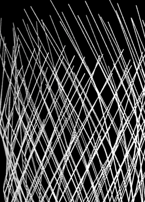
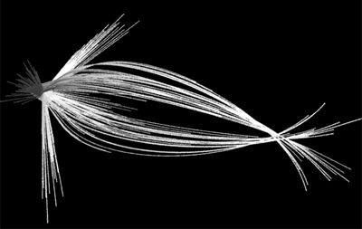
For example, figure 1 illustrates how particle positional data, when rendered as RenderMan curves, display the trajectories that were traced by the particles in the original particle system (figure 2).

The techniques shown on this page rely on the use of slim ribbox's and Tcl scripts. Example 1 serves as an introduction to the use of a ribbox that querries a particle system. The actual process of baking particle data is shown in example 2. The remaining examples demonstrate how the baked data can be used for different effects.

figure 1 - particle trajectories

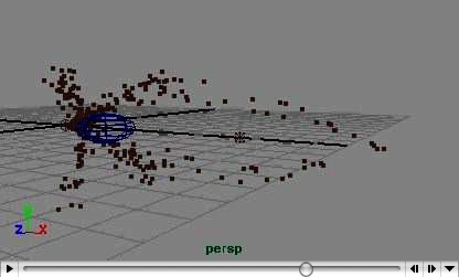
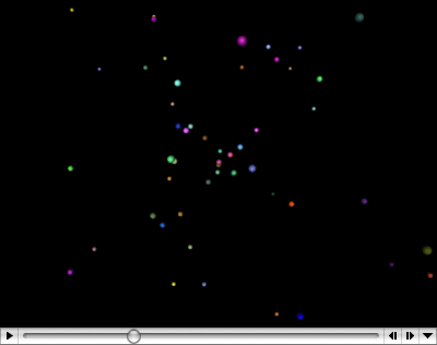
figure 2- original particle system

Example 1 - particle queries

Ribbox 1 lists a script that demonstrates the basics of querrying a particle system. The script would be attached the particles themselves, not to the emittor. As shown in a variety of ribbox examples (refer to 1 2 3 4), most MEL commands can be called via the built-in slim tcl procedure "clientcmd". For example, lines 2, 4 and 10 use MEL commands to querry the name of the shape node, the number of particles and their individual positions.

getParticleAttr returns an array of two strings. The built-in procedure "clientcmd" converts the array to a tcl list. The first item in the list is the name of the shape node. The xyz position of each particle is used to locate a randomly colored sphere.

The loop, lines 9 to 19, builds an output string that eventually contains a sequence of Rib statements that will cause prman to render the spheres that will "replace" the actual particles. The final rib statement, "Opacity 0 0 0", ensures the actual particles are invisible. Ideally, attribute "mtor invisibility" should be attached to the particles but it seems "mtor invis" does not work with particles - hence the hack of zero opacity!

figure 3

Of course, inserting colored spheres as substitutes for the actual Maya particles is of no importance. However, the script could be adapted to render rib archives. For example. the particle number (within the loop) could be used to cycle through a sequence of, say 25, numbered pre-baked ribs. Incidently, the following script assumes the pre-baked ribs have numeric extensions from "0000" to "0024". The slim variable $F is substituted by the frame number.

  set numExt [format %0.4d [expr (($n + $F) % 24)]]
  append ribout " ReadArchive \"PATH_TO_PREBAKES.$numExt.rib\"\n"

Figure 4 was produced by replacing lines 16 and 17 of the ribbox with the code shown above. Many thanks to Bryan Bentley of the Savannah College of Art and Design for the animation of the teapot that was used to generate 25 pre-baked ribs.

figure 4

Example 2 - baking particle positions

Ribbox listing 2 demonstrates how each particles positional data can be written (baked) to a series of text files. Each particle has its data saved to an individual file. Therefore, particles emitted early in an animation have more xyz positions than particles generated later in the animation. This is a rough and ready way of recording particle positions but it works quite well for moderately "light weight" particle systems.

The text shown in red must be edited to correspond to the directory in which the data files are to be saved.

A ribbox containing the (edited) text of listing 2 should be attached to a particle system. The renderer can be turned off using

    RenderMan Globals->Spool->Job Setup

Running the particle animation will generate a number of text files named particle.0000.rib, particle.0001.rib etc. A typical data file will contain listings of xyz positions, for example,

    0.0312244 0.00145994 -0.00867358
    0.143521 0.00671052 -0.0398675
    0.255817 0.0119611 -0.0710615
    0.368114 0.0172117 -0.102255
    0.48041 0.0224623 -0.133449

Example 3 - converting the data to curves

Once the particle data has been written it can be post-processed by a tcl script, or any other scripting language. Tcl listing 3, for example, converts the particle data into series of RenderMan curves - contained in a pre-baked rib file. For example, the 5 sets of xyz's shown above would define a curve in the following manner,

    Basis "b-spline" 1 "b-spline" 1
    Curves "cubic" [5] "nonperiodic"
    "P" [					
    0.0312244 0.00145994 -0.00867358
    0.143521 0.00671052 -0.0398675
    0.255817 0.0119611 -0.0710615
    0.368114 0.0172117 -0.102255
    0.48041 0.0224623 -0.133449					
    ]
    "constantwidth" [0.05]

The next listing is a tcl script that converts the xyz's in the data files into a rib file that defines curves whose CV's pass through each particle xyz positions.

figure 5

Ensure the items shown in blue conform to your directories.
Summary
    step 1 - create a particle system in maya,
    step 2 - attach the ribbox containing listing 2,
    step 3 - run the animation to produce the data files,
    step 4 - execute the tcl script (listing 4) to generate a pre-baked rib file.

Before referencing the baked rib file in maya it is best to check it with a simple rib file - rib listing . For example, in Cutter choose,

    Rman Tools->Docs->Single Frame Rib

Figure 5 shows part of a large "woven" set of curves. I grateful to Roberto Huacuja of the Savannah College of Art and Design for providing me with the particle system animation that generated the data.

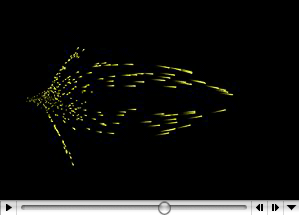
Figure 6 is an animation of a prebaked set of curves rendered with the shader shown in RSL listing 5. The shader progressively "moves" a patch of opacity along otherwise transparent curves. Sparky assumes the start and end of each flow line spans an "age" of 0.0 to 1.0. Of course this is wrong because the shorter lines represent the trajectories of young particles. Thus, the very short curves may only span an age of 0.9 to 1.0

figure 6 - animated shader (see figure 1)

Example 4 - converting the data to blobbies

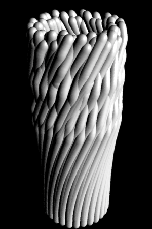
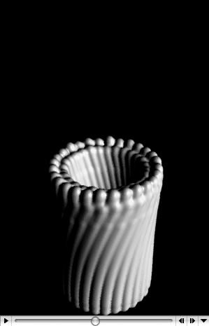
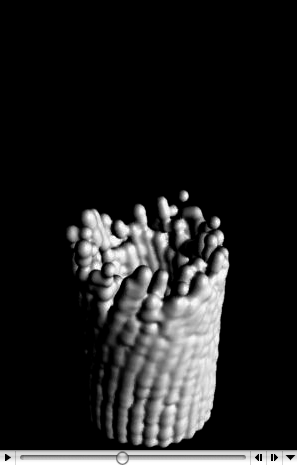
Figures 7, 8 and 9 are based on the data that produced figure 5.

Ribbox listing 6 converted the data files into approximately 150 Blobby's - each consisting of 88 "fused" ellipsoids.

Ribbox listing 7 is slightly more complex because not only does it produce a single Blobby (13776 "fused" ellipsoids shown in figure 8) but it can also animate the progress of the blobbing effect.

Figure 8 demonstrates the use of rand() to omit ellipsoids. The effect was achieved by substituting line 26 of listing 7 with the following code.

    if {[expr rand()] > 0.5} {
       lappend data $xyz
       }

figure 7 - see ribbox listing 6

figure 8 - see ribbox listing 7

figure 9 - see ribbox listing 7

1
2
3
4
5
6
7
8
9
10
11
12
13
14
15
16
17
18
19 
20
21
22
23
24
25
26
27
28
29
30
31
32
33
34
35
36

proc convertToMultiBlobby { datadir bakefile scale} {
   file delete -force $bakefile    
   set ribfile [open $bakefile w]
   set listing [glob -directory $datadir *]
   foreach item $listing {
      # will be reused to specify the full transform matrix
      set matrix "$scale 0 0 0  0 $scale 0 0  0 0 $scale 0 "
      # will list the blob codes and their offsets
      set blobOffsets "" 
      set blobIndices ""
      
        set datafile [open $item r]
      set blobData ""
      set count 0
       while { [eof $datafile] != 1 } {
         gets $datafile xyz
         if {[string length $xyz] > 0} {
            append blobData "$matrix $xyz 1\n"
            append blobOffsets "1001 [expr 16 * $count]\n"
            append blobIndices " $count"
            incr count
            }
         }
      set count [expr $count - 1]
      
      puts $ribfile "Blobby [expr $count + 1]"
      puts $ribfile "\[ $blobOffsets"
      puts $ribfile "0 [expr $count + 1] $blobIndices \]"
      puts $ribfile "\[ $blobData \]\n"
      puts $ribfile "\[\"\"\]"
      close $datafile
      }
   puts $count
   close $ribfile
   }
convertToMultiBlobby "G:/particle_data"  "G:baked_blobby.rib" 0.25

Ensure the items shown in blue conform to your directories.