RSL
Cellular Automata


return to main index


Introduction

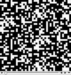
This tutorial presents the code for a shader that generates an animated pattern based on the principles of Conways Game of Life, so-called 2D cellular automata (CA). A full, or even a partial, discussion of cellular automata is beyond the scope of this tutorial. It is, therefore, assumed the reader has at least some familiarity with the basic concepts of CA. A static image of cellular automata is of little visual interest, only when animated does their complex behavior become apparent - figure 1.


Figure 1 (1.8 MB)


Cellular automata are generally displayed as a pattern of cells. The cells seen above are represented by the micropolygons into which prman has diced a surface. The 2 by 2 polygon shown above had a ShadingRate of 62 and was rendered using orthographic projection - listing 1. The shading rate yielded a pattern of 32 by 32 cells ie. micropolygons.


Listing 1 - celluar.rib


Option "searchpath" "shader" "@:PATH_TO_USERS_SHADERS"
DisplayChannel "float _cellLife"
Display "cellular" "it" "rgb"
Format 240 240 1
Projection "orthographic"
ShadingRate 62
  
Translate  0 0 3
Rotate -90 1 0 0
Rotate 0   0 1 0
Scale 1 1 -1
WorldBegin
    Attribute "dice" "rasterorient" 0 # view-independent dicing
    Surface "cellular"
            "float init" 1
            "float count" 32
            "string oldcell" ["./old.ptc"] # note "./"
            "string newcell" ["./new.ptc"]
    AttributeBegin
        Scale 2 2 2
        Polygon "P" [-0.5 0 -0.5  -0.5 0 0.5  0.5 0 0.5  0.5 0 -0.5]
                "st" [0 0  0 1  1 1  1 0]
    AttributeEnd
WorldEnd
System "cp new.ptc old.ptc"
System "rm ./new.ptc"


The Rules of the Game of Life

Each cell (ie. micropolygon) can be in one of two states, either alive or dead. White cells are those considered to be alive; black cells are those that are dead. The state of a cell, say at frame 10, depends on the state of the cells that surrounded it on frame 9. In short, a cell lives, dies or a dead cell becomes alive depending on how many of its neighbors, in the previous frame of animation, were alive (possible overpopulation) or dead (possible underpopulation). These are the rules of the game of life.


Shading Issues

Because the renderer cannot be queried about the "previous" condition of a micropolygon it is impossible, without some trickery, to implement a shader that mimics the behavior of cellular automata. However, point clouds provide an opportunity to record the condition of a micropolygon so that it can be queried in a subsequent frame of animation. The technique presented here relies on the use of two point clouds. From one point cloud, "old.ptc", it reads data that was baked during the previous frame of an animation. Into the other point cloud, "new.ptc", it writes data that will be used in the next frame of animation.


Algorithm

On the first frame of an animation the shader, for each micropolygon,

  1. randomly assigns it a state - black (dead) or white (alive),
  2. writes the state to "new.ptc".

On all subsequent frames, again for each micropolygon, the shader,

  1. reads "old.ptc" to query the state of a neighborhood of micropolygons,
  2. sets a new state according to the rules of the game of life,
  3. writes the state to "new.ptc".

After each frame of animation the data in "old.ptc" is overwritten by "new.ptc". Data written to a point cloud is "bound" to the shading point P and the surface normal N of a micropolygon. Reading a point cloud consists of referencing the baked data via P and N. To determine the state of a cell (micropolygon) a shader must query those cells (micropolygons) that were adjacent to it on the previous frame of animation. Since P is a (3D) point it is uncertain what values should be used to define the 8 vectors that will provide offsets by which the adjacent cells (micropolygons) can be referenced in the point cloud. To overcome this difficulty the shader presented here does not use P but instead, constructs a proxy point based on 's' and 't'.

Because the size of a micropolygon varies across a surface when viewed by a perspective camera a limitation of this approach is that an orthographic camera must be used to render a planar square polygon. Only in this way can a shader ensure it is accurately sampling a point cloud. Adaptive sampling was tried ie.

    float stepSize = sqrt(area(P));

but it gave poor results.

Listing 2 - cellular.sl


surface
cellular(float init = 1,     /* [0 or 1] Set to 1 for the first frame */
               count = 16;   /* Number of cells                       */
        string oldcell = "", /* Cell values from previous frame       */
               newcell = ""  /* Cell values for the current frame     */
              )
{
float    stepSize = 1/count;
float    halfStep = stepSize/2;
float    ss = s + halfStep;
float    tt = t + halfStep;
float    thisCurrLife;
float    thisPrevLife;
point    thisCellPos = point "world" (ss, 0, tt);
float    cellLife[8] = {0,0,0,0,0,0,0,0};
point    cellPos[8];    // neighborhood cell positions
normal   n = 0;        // no useful data for the normal
float    numLive = 0;
  
if(init)
    thisCurrLife = (random() > 0.61) ? 1 : 0;
  
if(init != 1 && oldcell != "") {
    // Determine the coordinates the cells in the immediate 
    // neighborhood of the current micropolygon. Note we wrap
    // to avoid attempting to access non existent cells.
    float sb = ss - stepSize;    // s back
    if(sb < 0) 
        sb = 1 - halfStep;
    
    float sf = ss + stepSize;     // s forward
    if(sf > 1)
        sf = halfStep;
        
    float tb = tt - stepSize;     // t back
    if(tb < 0)
        tb = 1 - halfStep;
        
    float tf = tt + stepSize;     // t forward
    if(tf > 1)
        tf = halfStep;
    
    cellPos[0] = point "world" (sb, 0, tb);
    cellPos[1] = point "world" (ss, 0, tb);
    cellPos[2] = point "world" (sf, 0, tb);
        
    cellPos[3] = point "world" (sb, 0, tt);
    cellPos[4] = point "world" (sf, 0, tt);
  
    cellPos[5] = point "world" (sb, 0, tf);
    cellPos[6] = point "world" (ss, 0, tf);
    cellPos[7] = point "world" (sf, 0, tf);
    
    // Query the value the current cell had in the previous frame
    // of animation.
    texture3d(oldcell, thisCellPos, n, "_cellLife", thisPrevLife);
  
    float j;
    // Query the value of neighbors and assign their values
    // to the cellLife array.
    for(j = 0; j < 8; j = j + 1) {
        texture3d(oldcell, cellPos[j], n, "_cellLife", cellLife[j]);
        }
    // Count the live cells.
    for(j = 0; j < 8; j = j + 1) {
        cellLife[j] = (cellLife[j] > 1.0) ? 1 : 0;
        if(round(cellLife[j]) == 1) {
            numLive = numLive + 1;
            }
        }
    // Apply the rules of life
    if(thisPrevLife > 1.0)
        thisPrevLife = 1;
    else
        thisPrevLife = 0;
    if(thisPrevLife == 1) {
        if(numLive == 2 || numLive == 3)
            thisCurrLife = 1;    // continue living
        else
            thisCurrLife = 0;    // become dead
        }
    if(thisPrevLife == 0) {
        if(numLive == 3)
            thisCurrLife = 1;    // birth
        else
            thisCurrLife = 0;    // remain dead
        }    
    }
if(newcell != "") {
    // Bake the value of the cell (micropolygon). Its bumped up
    // to ensure that any slight numeric inaccuracies ie. 0.99999
    // go way over 1.0000. This was an issue during the development
    // of the shader and its done here as a precaution!
    bake3d(newcell, "_cellLife", thisCellPos, n, "interpolate", 0,
                    "_cellLife", thisCurrLife * 2);
    }
Oi = Os;
Ci = Oi * thisCurrLife;
}


Trial and Error

Determining the value of the "count" shader parameter for a particular ShadingRate and Format is a matter of trial and error. For example, in listing 1 the Format was 240 240 1. Counting the cells in the rendered image it was determined the renderer had diced the surface into 32x32 micropolgons. Hence, the "count" parameter was set to 32. However, using,

    Format 300 300 1

generates an image with 40x40 cells.

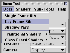
Using Cutter's keyframing facility (refer to the tutorial "Cutter: KeyFraming") an animation sequence is easily generated. For example, with the cellular.rib open in Cutter go to the Rman Tools and select the "Key Frame Rib" menu item - figure 2.


Figure 2


A sample keyframe file is shown below. Don't forget to set PATH_TO_USERS_SHADERS to the path to the directory into which your cellular.slo was compiled.


Listing 3 - cellular.key


Option "searchpath" "shader" "@:PATH_TO_USERS_SHADERS"
DisplayChannel "float _cellLife"
Format 300 300 1
ShadingRate 62
  
Display "cell_300" "tiff" "rgb"
Tween "from" 1 "to" 2 "frames" 600
Tween "output" "all"
  
KeyFrameBegin 1
    Projection "orthographic"
    Translate  0 0 3
    Rotate -90 1 0 0
    Rotate 0   0 1 0
    Scale 1 1 -1    
    WorldBegin
        Attribute "dice" "rasterorient" 0 # view-independent dicing
        Surface "cellular"
                "float init" 1
                "float count" 40
                "string oldcell" ["./old.ptc"] # note ./
                "string newcell" ["./new.ptc"]
        AttributeBegin
            Scale 2 2 2
            Polygon "P" [-0.5 0 -0.5  -0.5 0 0.5  0.5 0 0.5  0.5 0 -0.5]
                    "st" [0 0  0 1  1 1  1 0]
        AttributeEnd
    WorldEnd
    System "cp new.ptc old.ptc"
KeyFrameEnd
  
KeyFrameBegin 2
    Projection "orthographic"    
    Translate  0 0 3
    Rotate -90 1 0 0
    Rotate 0   0 1 0
    Scale 1 1 -1
    WorldBegin
        Attribute "dice" "rasterorient" 0 # view-independent dicing
        Surface "cellular"
                "float init" 0
                "float count" 40
                "string oldcell" ["./old.ptc"] # note ./
                "string newcell" ["./new.ptc"]    
        AttributeBegin
            Scale 2 2 2
            Polygon "P" [-0.5 0 -0.5  -0.5 0 0.5  0.5 0 0.5  0.5 0 -0.5]
                    "st" [0 0  0 1  1 1  1 0]
        AttributeEnd
    WorldEnd
    System "cp new.ptc old.ptc"
KeyFrameEnd

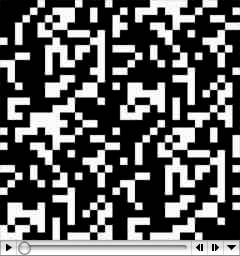
The animation generated by cellular.key is shown below.


Figure 3 (3.3 MB)


© 2002- Malcolm Kesson. All rights reserved.