RSL
Writing Displacement Shaders

return to main index

Overview

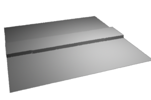
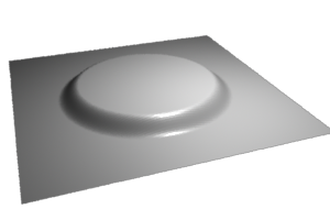
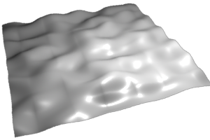
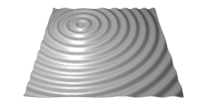
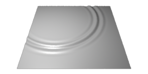
Displacement shaders alter the smoothness of a surface, however, unlike bump mapping which mimics the appearance of bumpiness by reorientating surface normals, displacement shading genuinly effects the geometry of a surface. In the case of Pixars prman renderer, each object in a 3D scene is sub-divided into a fine mesh of micro-polygons after which, if a displacement shader has been assigned to an object, each micro-polygon is "pushed" or "pulled" in a direction that is parallel to the original surface normal of the micro-polygon. After displacing the micro-polygon the orientation of the local surface normal (N) is recalculated.

Figure 1

The following algorithm lists the four basic steps that a displacement shader generally follows in order to set the position (P) and normal (N) of the micro-polygon being shaded.

To make a meaningful decision about the distance, if any, a micro-polygon should be displaced, a shader may make reference to the micro-polygon's,

• 2D surface position s, t, u, v,
• 3D xyz position P,
• orientation N,
• camera distance L.

plus other less obvious attributes of a micro-polygon. Such information is either directly or indirectly available in data the renderer makes available to a shader through the use of global variables.

Displacement Shaders & Global Variables

The following table lists the global variables accessible to a displacement shader. For the corresponding list of global variables available to a surface shader refer to the tutorial "RSL: What is a Surface Shader".

Using Cutter for Shader Writing

It is highly recommended the reader use Cutter for their shader writing. It has many very useful time saving features. Refer to the tutorial "Cutter: Shader Writing" for information about Cutter and how it should be set up.

Basic Code

The experiments on displacement shading in this tutorial are based the shader shown in listing 1.

Listing 1

displacement 
test1(float Km = 0.1)
{
float   hump = 0;
normal  n;
  
/* STEP 1 - make a copy of the surface normal */
n = normalize(N);
  
/* STEP 2 - calculate the displacement */
hump = 0;
  
/* STEP 3 - assign the displacement to P */
P = P - n * hump * Km;
  
/* STEP 4 - recalculate the surface normal */
N = calculatenormal(P);
}

Texture Coordinates

Although micro-polygons have 3D xyz positions, given by the global variable P, they also have a 2D position in 'st' texture space. Irrespective of their actual size, nurbs and quadric surfaces cover exactly 1 unit in 's' and 't'.

Figure 2

Use Cutter's Rman Tool palette to generate a rib file to test your shaders - figure 3. The poly-plane is set up to also cover one unit in texture space ie.

    Polygon "P"  [-0.5 0 -0.5  -0.5 0 0.5  0.5 0 0.5  0.5 0 -0.5] 
            "st" [0 0  0 1  1 1  1 0]

Figure 3

The first shader, listing 2, uses a simple "if" test to decide whether a micro-polygon is within a narrow band.

Listing 2

displacement 
test2(float Km = 0.1)
{
float   hump = 0;
normal  n = normalize(N);
  
if(t >= 0.4 && t <= 0.6)
    hump = 1;
  
P = P - n * hump * Km;
N = calculatenormal(P);
}

Figure 4

The edge of the raised band is aliased. For the moment we will ignore the defect. The next shader uses the RSL distance() function to determine if a micro-polygon is within a distance defined by the shader parameter radius.

Listing 3

displacement 
test3(float Km = 0.1,
            radius = 0.3)
{
float   hump = 0;
normal  n = normalize(N);
float   d = distance(point(0.5,0.5,0), point(s, t, 0));
  
if(d <= radius)
    hump = 1;
  
P = P - n * hump * Km;
N = calculatenormal(P);
}

Again, the aliased rim of the circle will be ignored.

Figure 5

Smoothstep

The shader in listing 4 uses the RSL smoothstep() function to soften the edge of the circular displacement. It also provides an extra shader parameter to control the width of the softening. For more information about the use of the smoothstep() function refer to the tutorial "RSL: Using Smoothstep".

Listing 4

displacement 
test4(float Km = 0.1,
            radius = 0.3,
            blur = 0.04)
{
float   hump = 0;
normal  n = normalize(N);
float    d = distance(point(0.5,0.5,0), point(s, t, 0));
  
hump = 1 - smoothstep(radius - blur, radius + blur, d);
  
P = P - n * hump * Km;
N = calculatenormal(P);
}

Figure 6

Listing 5 provides additional parameters, s_center and t_center, to control the placement of the circle.

Listing 5

displacement 
test5(float Km = 0.1,
            radius = 0.1,
            blur = 0.04,
            s_center = 0.25,
            t_center = 0.25)
{
float   hump = 0;
normal  n = normalize(N);
float   d = distance(point(s_center,t_center,0),point(s,t,0));
  
hump = 1 - smoothstep(radius - blur, radius + blur, d);
  
P = P - n * hump * Km;
N = calculatenormal(P);
}

Figure 7

Displacement Mapping

The shader in listing 6 implements simple image embossing. Although the texture() can return a float the value represents only the red channel of the image. Unfortunately, it is not an average of the "rgb" channels. For this reason the shader calculates the average "rgb" value. Strickly speaking, the shader should calculate the grayscale value but taking a simple average is good enough.

Listing 6

displacement 
test6(float Km = 0.1;
     string texname = "")
{
float   hump = 0;
normal  n = normalize(N);
  
if(texname != "") {
    color c = texture(texname);
    hump = (comp(c, 0) + comp(c, 1) + comp(c, 2))/3;
    }
  
P = P - n * hump * Km;
N = calculatenormal(P);
}

Figure 8

The shader was used in the rib file in the following way.

    Displacement "test6" "texname" ["swazi.tx"] "Km" -0.20

The texture file "swazi.tex" was converted from the image shown in figure 9. For more information about converting tif files to textures refer to the tutorial "Writing Surface Shaders".

Figure 9

Noise I

The next shader uses the RSL noise() function to create a bumpy surface. For more information about this function refer to the tutorials "Using Noise" and "Writing Surface Shaders".

Listing 7

displacement 
test7(float Km = 0.1,
            s_freq = 6,
            t_freq = 8)
{
float   hump = 0;
normal  n = normalize(N);
  
hump = noise(s * s_freq, t * t_freq);
  
P = P - n * hump * Km;
N = calculatenormal(P);
}

Figure 10

Because the inputs to the noise() function are 's' and 't' the bumps are "parented" to the texture space of the surface and as such will move with the object. In other words the bumps will not appear to slide or move over the surface. If movement of the bumps is required it can be done in two ways. Listings 8 and 9 address this issue.

Animated 'st' Noise

The shader in listing 8 applies an offset to the 's' and 't' values before they are scaled by their respective frequency parameters. The bumps can be animated incremently increasing the s_offset and/or t_offset on a frame-by-frame basis. For information about Cutter's keyframing capabilities refer to the tutorial "KeyFraming"

Listing 8

displacement 
test8(float Km = 0.1,
            s_freq = 6,
            s_offset = 0,
            t_freq = 8,
            t_offset = 0)
{
float   hump = 0;
normal  n = normalize(N);
  
hump = noise((s - s_offset) * s_freq, 
             (t - t_offset) * t_freq);
  
P = P - n * hump * Km;
N = calculatenormal(P);
}

The banding seen in figures 11 and 12 are caused by a defect in the (Perlin) noise function. In theory the displacements should be smooth in all directions but there are discontinuities at the integer lattice. The defect is particularly noticable with large displacements.

Figure 11
s_offset = 0.0

Figure 12
s_offset = 0.1

Animated 3D Noise

The shader in listing 9 uses a micro-polygons xyz position (P) as an input to noise(). Unlike the previous shader in listing 8 that supplied two inputs, and hence produced 2D noise, the current shader generates true 3D noise. The shader was applied to a cubic stack of poly-planes from which a spherical hole "gouged out" with a special purpose surface shader. The variations in displacement caused by the 3D noise can clearly be seen.

Figure 13

Listing 9

displacement 
test9(float Km = 0.1,
             freq = 1)
{
float   hump = 0;
normal  n = normalize(N);
  
hump = noise(P * freq);
  
P = P - n * hump * Km;
N = calculatenormal(P);
}

The principle issue with the shader is that point 'P' is defined in "camera space". Consequently, the noise is "parented" to the camera - movements of the camera will move the noise! Refer to the tutorial "Writing Surface Shaders" for a more information about coordinate systems.

To ensure an artist has control over 3D noise the next shader enables point 'P' to be transformed into either a pre-existing or a user-defined coordinate system. The pre-existing coordinate systems are "camera", "world", "object" and "shader". However, as shown next a user-defined coordinate system can be established with the CoordinateSystem rib statement.

Listing 10a

displacement 
test10(float Km = 0.1,
             freq = 1;
    string   space = "object")
{
float   hump = 0;
normal  n = normalize(N);
  
point    p = transform(space, P);
hump = noise(p * freq);
  
P = P - n * hump * Km;
N = calculatenormal(P);
}

Figure 14

    Displacement "test10" "space" ["object"]

Figure 15

    Displacement "test10" "space" ["myspace"]

The rib file used to render figure 15 defined a user-defined coordinate system as follows.

Listing 10b

    TransformBegin
        Translate 0 0 0
        Rotate  0 1 0 0
        Rotate  0 0 1 0
        Rotate  0 0 0 1
        Scale   0.25 1 1
        CoordinateSystem "myspace"
    TransformEnd
    Displacement "test10" "space" ["myspace"] "Km" -0.50 "freq" 1 

Turbulance

A simulation of turbulance or fractal noise can be achieved by using the noise() within a loop. On each iteration of the loop the value returned from noise() is added to the result of the previous iteration. Successfully higher frequencies but smaller amplitudes are used for iteration. The visual result is richer because the shading can appear to mimic natural surfaces ie. large bumps have small bumps which in turn have enen smaller

Listing 11a

displacement 
test11a(float Km = 0.1,
              freq = 1,
              layers = 3;
    string   space = "object")
{
float   hump = 0;
normal  n = normalize(N);
point   p = transform(space, P);
float   j, f = freq, amplitude = 1;
 
for(j = 0; j < layers; j += 1) {
    hump += noise(p * f) * amplitude;
    f *= 2;
    amplitude *= 0.5;
    }
  
P = P - n * hump * Km;
N = calculatenormal(P);
}

The problem with applying a displacement directly with the value returned from noise() is that the displaced surface moves away from its original position. This "side-effect" is made worse when a number of displacements are summed. For example, in figure 16 the lower poly-plane marks the starting position for the displaced polygon. In figure 17 an adjustment has been made to the shader so that on average the displaced surface is 50% above and below its original location.

Figure 16

Figure 17

In listing 11b a constant value of 0.5 is substracted from the noise value. In general it is a good idea to always subtract 0.5 from noise.

Listing 11b

displacement 
test11b(float Km = 0.1,
             freq = 1,
             layers = 3;
    string   space = "object")
{
float   hump = 0;
normal  n = normalize(N);
point   p = transform(space, P);
float   j, f = freq, amplitude = 1;
  
for(j = 0; j < layers; j += 1) {
    hump += (noise(p * f) - 0.5) * amplitude;
    f *= 2;
    amplitude *= 0.5;
    }
  
P = P - n * hump * Km;
N = calculatenormal(P);
}

Figure 18
From left to right - "layers" 3, "layers" 4 and "layers" 5

Some interesting visual effects can also be created by ensuring the value returned from noise() is always positive. Listing 11c uses the abs() function to create the effect seen in figure 19.

Listing 11c

displacement 
test11c(float Km = 0.1,
              freq = 1,
              layers = 3;
    string    space = "object")
{
float   hump = 0;
normal  n = normalize(N);
point   p = transform(space, P);
float   j, f = freq, amplitude = 1;
  
for(j = 0; j < layers; j += 1) {
    hump += abs(noise(p * f) - 0.5) * amplitude;
    f *= 2;
    amplitude *= 0.5;
    }
  
P = P - n * hump * Km;
N = calculatenormal(P);
}

Figure 19

Ripples

Listing 3 demonstrated the use of the RSL distance() function to calculate the distance between to points. Figure 20 shows a method that uses the theorem of Pythagoras to also calculate the straight line distance between two points. One point is defined by the coordinates a,b and the other by s,t. In listing 12 the first coordinates will define the center of a ripple while the second coordinates are those for the micro-polygon that is being shaded.

Listing 12a

displacement ripple1(float Km = 0.03, 
                           numripples = 8,
                           a = 0.3, 
                           b = 0.25)
{ 
float  sdist = s - a,
       tdist = t - b,
       dist = sqrt(sdist * sdist + tdist * tdist),
       hump = sin(dist  * 2 * PI * numripples);
 
normal n = normalize(N);
    
P = P - n * hump * Km;
N = calculatenormal(P);
}

Figure 20

Ripples in a pool of water, say as the result of a drop of rain, normally propogate outward as 2 or 3 concentric waves. Listing 12b applies a constraint on the ripples seen in figure 20 in order to mimic the rain-drop effect. The constraint is based on a double use of the smoothstep() function. For more information about this RSL function refer to the tutorial "RSL: Using smoothstep".

Listing 12b

displacement ripple1(float Km = 0.03, 
                           numWaves = 12,
                           a = 0.3, 
                           b = 0.25,
                           rippleRad = .5,
                           rippleWidth = 0,
                           rippleFade = 0.13)
{ 
float  sdist = s - a,
       tdist = t - b,
       dist = sqrt(sdist * sdist + tdist * tdist),
       hump = sin(dist  * 2 * PI * numWaves);
  
float  w = rippleWidth/2;
float  inner = rippleRad - w;
float  outer = rippleRad + w;
hump = hump * smoothstep(inner - rippleFade, inner, dist) * 
            (1 - smoothstep(outer, outer + rippleFade, dist));
normal n = normalize(N);
    
P = P - n * hump * Km;
N = calculatenormal(P);
}

Figure 21